Fitting a Bayesian Factor Analysis Model in Stan
By Rick Farouni
The Ohio State University
04/26/2015
Model Specification
Let \({\mathbf{y}}^{\intercal}=(y_{1}, y_{2},..., y_{P})\) be an observable P-dimensional random vector and let \({\boldsymbol{\theta}}\) be a D-dimensional random vector of latent traits that probabilistically determine the observable responses. A factor analysis model with factor loading matrix \({\boldsymbol{\Lambda}}\), latent trait correlation matrix \({\boldsymbol{\Phi}}\), and diagonal covariance matrix \({\boldsymbol{\Psi}}\) for the errors \({\boldsymbol{\varepsilon}}\) can be written as
\[ \begin{align} \\ &{\mathbf{y}}={\boldsymbol{\Lambda}}{\boldsymbol{\theta}}+ {\boldsymbol{\varepsilon}}\\ \end{align} \]
where \[ \begin{align} \begin{pmatrix} {\boldsymbol{\theta}}\\ {\boldsymbol{\varepsilon}}\end{pmatrix} \sim &Normal\Bigl(\textbf{0},\begin{bmatrix}{\boldsymbol{\Phi}}& \textbf{0} \\ \textbf{0} & {\boldsymbol{\Psi}}\end{bmatrix}\Bigr) \end{align} \]
and
\[ \begin{align} {\boldsymbol{\Lambda}}= \begin{bmatrix} \lambda_{1,1}& ...& \lambda_{1,D}\\ \lambda_{2,1}& ...& \lambda_{2,D}\\ \vdots & \vdots & \vdots \\ \lambda_{p,1} & ...& \lambda_{P,D}\\ \end{bmatrix} {\boldsymbol{\Phi}}_{D} = \begin{bmatrix} 1 & \varphi_{1,2} & ...& \varphi_{1,D} \\ \varphi_{2,1} & 1 & ... & \varphi_{2,D}\\ \vdots & \vdots & \vdots & \vdots \\ \varphi_{D,1} & ...& \varphi_{D,D-1} & 1 \end{bmatrix} \quad {\boldsymbol{\Psi}}_{P} = \begin{bmatrix} \psi_1& 0 & ...& 0 \\ 0 & \psi_2 & ... & 0\\ \vdots & \vdots & \vdots & \vdots \\ 0 & 0 & ... & \psi_p \end{bmatrix} \end{align} \]
or equivalently as
\[ \begin{align} {\mathbf{y}}\sim & Normal_{p}(\textbf{0},{\boldsymbol{\Lambda}}{\boldsymbol{\Phi}}{\boldsymbol{\Lambda}}^{\intercal}+{\boldsymbol{\Psi}}) \end{align} \]
Note that \({\boldsymbol{\Psi}}\) is diagonal since the assumption of local item independence entails that the partial covariance of any two latent responses given the latent traits equals zero, which in turn implies that the elements of \({\boldsymbol{\varepsilon}}\) are themselves uncorrelated (Lord & Novick, 1968).
For N observations sampled from a single homogeneous population, the joint posterior distribution is then
\[ \begin{align} p(\boldsymbol{\Theta},{\boldsymbol{\Lambda}},\boldsymbol{\tilde{\xi}},\boldsymbol{{\boldsymbol{\Phi}}}\mid {\mathbf{Y}})\propto & \biggl[\prod_{n=1}^N\ p({\mathbf{y}}_{n}\vert\boldsymbol{\theta_n,}{\boldsymbol{\Lambda}})\biggr] \biggl[\prod_{n=1}^N\ p\left(\boldsymbol{\theta}_{n}\mid \boldsymbol{{\boldsymbol{\Phi}}}\right)\biggr] p\left({\boldsymbol{\Lambda}}\mid \boldsymbol{\tilde{\xi}}\right) p(\boldsymbol{{\boldsymbol{\Phi}}})p(\boldsymbol{\tilde{\xi}}) \end{align} \]
where \(\boldsymbol{\Theta}=\left(\boldsymbol{\theta_1},\boldsymbol{\theta_2},... \boldsymbol{\theta_n},... \boldsymbol{\theta_N}\right)\). Moreover, by intergrating out the N D-dimensional latent vectors, we obtain the marginalized posterior
\[ \begin{align*} p({\boldsymbol{\Lambda}},\boldsymbol{\tilde{\xi}},\boldsymbol{{\boldsymbol{\Phi}}}\mid {\mathbf{Y}})\propto & \biggl[ \prod_{n=1}^N \int_{R_{{\boldsymbol{\vartheta}}}}p({\mathbf{y}}_{n}\vert\boldsymbol{\theta_n,}{\boldsymbol{\Lambda}}) p\left(\boldsymbol{\theta}_{n}\mid \boldsymbol{{\boldsymbol{\Phi}}}\right) d\boldsymbol{\theta} \biggr] p\left({\boldsymbol{\Lambda}}\mid \boldsymbol{\tilde{\xi}}\right) p(\boldsymbol{{\boldsymbol{\Phi}}})p(\boldsymbol{\tilde{\xi}}) \end{align*} \]
Here, \({\mathbf{y}}_{n}\) is a \(P\)-dimensional vector of responses for respondent \(n\).
Identification
We say that a model is not identified if there are two or more distinct parameter points that can generate the same joint probability distribution. For example, if we can find a matrix not equal to , such that the two distinct set of parameters \(({\boldsymbol{\Lambda}},{\boldsymbol{\Phi}})\) and \(({\boldsymbol{\Lambda}}^\bigstar,{\boldsymbol{\Phi}}^\bigstar)\) define the same probability distribution
\[ \begin{align*} {\mathbf{y}}\sim &Normal\Bigl(\textbf{0},{\boldsymbol{\Lambda}}{\boldsymbol{\Phi}}{\boldsymbol{\Lambda}}^{\intercal}+{\boldsymbol{\Psi}}\Bigr)\\ \equiv &Normal\Bigl(\textbf{0},({\boldsymbol{\Lambda}}\textbf{T}) ({\textbf{T}}^{-1}\bigl({\boldsymbol{\Phi}}\bigr){{\textbf{T}}^{\intercal^{-1}}})({\textbf{T}}^{\intercal}{\boldsymbol{\Lambda}}^{\intercal})+{\boldsymbol{\Psi}}\Bigr)\\ \equiv&Normal\Bigl(\textbf{0},{\boldsymbol{\Lambda}}^\bigstar{\boldsymbol{\Phi}}^\bigstar{\boldsymbol{\Lambda}}^{\bigstar^\intercal}+{\boldsymbol{\Psi}}\Bigr) \end{align*} \]
then it follows then that the model is not identified. Conceptually, think of the latent variables \({\boldsymbol{\theta}}\) as spanning a \(D\)-dimensional space, the latent space, and any combination of the traits that define a particular person \(p\) can be represented by a point residing in that space. However, since \({\boldsymbol{\theta}}\) is latent, it has no frame of reference (and \({\mathbf{y}}\) as well). To establish a frame of reference, we need to specify a point of origin, a unit of measurement or scale, a set of D basis vectors that define the coordinates and the direction. These indeterminacies correspond to location, scale, rotation, and reflection invariance and to label switching if the basis vectors are not ordered.
Scale and Location Invariance
To specify a metric of measurement, we need to set the location and scale of the latent variables in the model. For \({\boldsymbol{\theta}}\) the location and scale were determined by specifying the means to zero and the variances to 1.
Rotation Invariance
Parameters are said to be invariant under rotation when we can find an orthogonal rotation matrix \(\textbf{T}\), where \(\textbf{T}^{\intercal}\textbf{T}={\boldsymbol{\Phi}}=\mathbf{I}\), such that when we rotate \({\boldsymbol{\Lambda}}\) and \({\boldsymbol{\theta}}\), we obtain two rotated matrices \({\boldsymbol{\Lambda}}^{\ast}={\boldsymbol{\Lambda}}\textbf{T}^{\intercal}\) and \({\boldsymbol{\theta}}^{\ast}=\textbf{T}{\boldsymbol{\theta}}\) whose product gives us back the original matrices
\[ \begin{align*} {\boldsymbol{\Lambda}}^{\ast}{\boldsymbol{\theta}}^{\ast}={\boldsymbol{\Lambda}}\textbf{T}^{\intercal}\textbf{T}{\boldsymbol{\theta}}={\boldsymbol{\Lambda}}{\boldsymbol{\theta}}\end{align*} \]
In factor analysis, there are two approaches to deal with rotational invariance. In Exploratory Factor Analysis (Thurstone, 1947), we set \({\boldsymbol{\Phi}}=\textbf{I}\) to make \({\boldsymbol{\Lambda}}{\boldsymbol{\Lambda}}^{\intercal}\) identifiable and chose \({\boldsymbol{\Lambda}}\) such that it meets certain criteria for interpretability. For example, one criterion, the VARIMAX criterion (Kaiser, 1958), finds a simple interpretable solution by rotating the factors so that each factor has a large number of loadings with values near zero and small number of loadings with large values. Note that, the resulting rotated matrix is not unique. For a \(D\)-dimensional model, there are still \(2^D \times D!\) matrices in its equivalence class. We should add that, that label switching (i.e., column permutations) and sign reversals are not considered a problem in the frequentist framework because inference can be restricted to one likelihood mode with the proper choice of initial values. Moreover, after applying a rotation criterion, the common practice is that the researcher usually flips the signs and orders the \(D\) columns of the orthogonally rotated loading matrix to obtain the most interpretable solution among the \(2^D \times D!\) possible matrices that satisfy the rotation criterion used.
In the second approach, Confirmatory Factor Analysis (Joreskog, 1973), the off-diagonal elements of \({\boldsymbol{\Phi}}\) are allowed to be unconstrained and the rotational invariance of \({\boldsymbol{\Lambda}}\) and \({\boldsymbol{\Phi}}\) is resolved by imposing theoretically informed constraints on \({\boldsymbol{\Lambda}}\). If no constraints are imposed on \({\boldsymbol{\Lambda}}\), then we can find a transformation matrix \(\textbf{T}\) with the constraint
\[\operatorname{Diag}({\boldsymbol{\Phi}})=\operatorname{Diag}({\textbf{T}}^{-1}{\textbf{T}}^{\intercal^{-1}})=\mathbf{I}\]
such that
\[ \begin{align*} {\boldsymbol{\Lambda}}{\boldsymbol{\Phi}}{\boldsymbol{\Lambda}}^{\intercal}=({\boldsymbol{\Lambda}}\textbf{T}) ({\textbf{T}}^{-1}{\boldsymbol{\Phi}}{\textbf{T}}^{\intercal^{-1}})({\textbf{T}}^{\intercal}{\boldsymbol{\Lambda}}^{\intercal}) \end{align*} \]
Note that although the transformation matrix is referred in the literature as an oblique rotation matrix (Browne, 2001), it is not necessarily orthogonal and therefore not exactly a rotation matrix.
Identification Conditions
(Anderson & Rubin, 1956) suggested that model identification can be achieved by imposing at least \(D^2\) restrictions on \(({\boldsymbol{\Lambda}},{\boldsymbol{\Phi}})\). (Howe, 1955) stated three sufficient conditions for local uniqueness of \({\boldsymbol{\Lambda}}\) and recently added a fourth condition to insure global rotational uniqueness. To ensure uniqueness according to the four conditions, we need to
- Make \({\boldsymbol{\Phi}}\) a positive definite correlation matrix such that \(\operatorname{Diag}({\boldsymbol{\Phi}})= \mathbf{I}\)
- Fix at least \(D-1\) zeros in every column of \({\boldsymbol{\Lambda}}\)
- Check that the submatrix \(\mathbf{\Lambda_{d}}\) has rank \(D-1\), where \(\mathbf{\Lambda_{d}}\) is the matrix remaining after keeping the rows that have zero fixed entries in column \(d\), for all columns \(d=1,.., D\).
- Constrain one parameter in each column of \({\boldsymbol{\Lambda}}\) to take only positive or negative values.
Note that the first condition imposes \(D\) restrictions and the second condition imposes another\(D(D-1)\) constraints for a total of \(D^2\) constraints. Jointly, the first three conditions reduce the number of possible modes from infinitely many to just the \(2^D\) modes produced by sign reversals. The fourth condition further reduces that number to 1 so that the resulting parameter space is unimodal on the condition that the remaining parameters in the model are identified. At any rate, if we are not sure whether our specified constraints make the parameters locally identifiable, we can check for local identification algebraically by using the Wald Rank Rule that evaluates the rank of the Jacobian (Bekker, 1989) or if we are conducting maximum likelihood based analysis, we can empirically assess local identification from the quality of the information matrix produced by the computer model fit.
The Problematic Consequences of Imposing Constraints
Although some parameter constraints can guarantee a unimodal likelihood, they can have the unintended consequence of impacting the shape of the likelihood. In particular, the constraints can induce local modes in the likelihood and make estimation problematic. For example, (Millsap, 2001) has shown that some common constraint choices can produce a discrimination or loading matrix that lies outside the true equivalence class. Moreover, in maximum likelihood estimation, fixing the D(D-1)/2 elements to nonzero constants renders the large sample normal approximation inappropriate (Loken, 2005). But that is not all. Another consequence is that since the constraints are placed on particular elements of the parameter matrix, both estimation and inference will depend on the ordering of the variables in data matrix. Sometimes however, restricted confirmatory model estimation is not so problematic. For example, if our data is very informative and we restrict the factors to be orthogonal and we constrain D(D-1)/2 elements of \({\boldsymbol{\Lambda}}\) to zero while observing the rank condition (Algina, 1980), then the modes will most likely be separated, allowing us to obtain valid estimates of the standard errors of the loadings based on a unimodal normal approximation(Dolan & Molenaar, 1991).
For more information about model identification, you can check my earlier post hereSimulate Data
Using R, we generate data for a 3 dimensional latent factor model with 10 dimensional obsevation vector. We first set the random-number generator seed in order to make the results reproducible. We also load the package MASS to sample observations from a multivariate normal. We generate 300 observation vectors.
library("MASS")
set.seed(42)
D <-3
P <- 10
N <-300

mu_theta <-rep(0,D) # the mean of eta
mu_epsilon<-rep(0,P) # the mean of epsilon
Phi<-diag(rep(1,D))
Psi <- diag(c(0.2079, 0.19, 0.1525, 0.20, 0.36, 0.1875, 0.1875, 1.00, 0.27, 0.27))
l1 <- c(0.99, 0.00, 0.25, 0.00, 0.80, 0.00, 0.50, 0.00, 0.00, 0.00)
l2 <- c(0.00, 0.90, 0.25, 0.40, 0.00, 0.50, 0.00, 0.00, -0.30, -0.30)
l3<-  c(0.00, 0.00, 0.85, 0.80, 0.00, 0.75, 0.75, 0.00, 0.80, 0.80)
L <-cbind(l1,l2,l3) # the loading matrix

Theta <-mvrnorm(N, mu_theta, Phi) # sample factor scores
Epsilon <-mvrnorm(N, mu_epsilon, Psi) # sample error vector
Y<-Theta%*%t(L)+Epsilon# generate observable data
Let’s visualise the data
library("rbokeh")
df<-data.frame(Y)
tools <- c("pan", "wheel_zoom", "resize", "reset")
nms <- expand.grid(names(df)[1:P], rev(names(df)[1:P]), stringsAsFactors = FALSE)
nms$yaxis <- rep(c(TRUE, rep(FALSE, P-1)), P)
nms$xaxis <- c(rep(FALSE, (P-1)*P), rep(TRUE, P))
nms$h <- nms$w <- 75
nms$h[nms$xaxis] <- nms$w[nms$yaxis] <- 90
splom_list <- vector("list", P^2)

for(i in seq_along(splom_list)) {
   splom_list[[i]] <- figure(width = nms$w[i], height = nms$h[i],
    tools = tools, min_border = 2) %>%
    ly_points(nms$Var1[i], nms$Var2[i], data = df,
       size = 1) %>%
    x_axis(visible = nms$xaxis[i], axis_label_text_font_size = "5pt") %>%
    y_axis(visible = nms$yaxis[i], axis_label_text_font_size = "5pt")
}

grid_plot(splom_list, nrow = P, ncol = P, same_axes = TRUE, link_data = TRUE)
Fit Model
In the unrestricted model, we have \(2^3=8\) possible column sign changes and \(3!=6\) column permutations, for a total \((8\times 6=48)\) matrices in the equivalence class. To obtain a single solution, we resticting the upper traingluar elements of L to zero, the diagnoal elements to be positive, and provide stan intial values for the parameters such that intial values are close to each other for all 4 chains. The stan model we are going to fit to the generated data puts a cauchy priors on the parameters. We also fit the model hierarchically so that the posterior won’t be sensitive to the choice of priors we have. We let the data estimate the hyperparameters! Here are the priors:
\[ \begin{align*} \operatorname{Diag}(\Psi) \sim & \textrm{Half-Cauchy}(\mu_{\psi},\sigma_{\psi}) \\ \operatorname{Diag}(L) \sim &\textrm{Half-Cauchy}(0,3)\\ \operatorname{Vech}(L) \sim &\textrm{Cauchy}(\mu_{L_t},\sigma_{L_t}) \end{align*} \]
where \(\operatorname{Vech}\) is the half-vectorization operator.
And the hyperpriors
\[ \begin{align*} \mu_{\psi}\sim &\textrm{Half-Cauchy}(0,1) \qquad &\sigma_{\psi}\sim \textrm{Half-Cauchy}(0,1)\\ \mu_{L_t} \sim &\textrm{Cauchy}(0,1) \qquad &\sigma_{L_t}\sim \textrm{Half-Cauchy}(0,1) \end{align*} \]
Stan Model Code
data {
  int<lower=1> N;                // number of
  int<lower=1> P;                // number of
  matrix[N,P] Y;                 // data matrix of order [N,P]
  int<lower=1> D;              // number of latent dimensions
}
transformed data {
  int<lower=1> M;
  vector[P] mu;
  M  <- D*(P-D)+ D*(D-1)/2;  // number of non-zero loadings
  mu <- rep_vector(0.0,P);
}
parameters {
  vector[M] L_t;   // lower diagonal elements of L
  vector<lower=0>[D] L_d;   // lower diagonal elements of L
  vector<lower=0>[P] psi;         // vector of variances
  real<lower=0>   mu_psi;
  real<lower=0>  sigma_psi;
  real   mu_lt;
  real<lower=0>  sigma_lt;
}
transformed parameters{
  cholesky_factor_cov[P,D] L;  //lower triangular factor loadings Matrix
  cov_matrix[P] Q;   //Covariance mat
{
  int idx1;
  int idx2;
  real zero;
  zero <- 0;
  for(i in 1:P){
    for(j in (i+1):D){
      idx1 <- idx1 + 1;
      L[i,j] <- zero; //constrain the upper triangular elements to zero
    }
  }
  for (j in 1:D) {
      L[j,j] <- L_d[j];
    for (i in (j+1):P) {
      idx2 <- idx2 + 1;
      L[i,j] <- L_t[idx2];
    }
  }
}
Q<-L*L'+diag_matrix(psi);
}
model {
// the hyperpriors
   mu_psi ~ cauchy(0, 1);
   sigma_psi ~ cauchy(0,1);
   mu_lt ~ cauchy(0, 1);
   sigma_lt ~ cauchy(0,1);
// the priors
  L_d ~ cauchy(0,3);
  L_t ~ cauchy(mu_lt,sigma_lt);
  psi ~ cauchy(mu_psi,sigma_psi);
//The likelihood
for( j in 1:N)
    Y[j] ~ multi_normal(mu,Q);
}
Now we fit the model to the data.
library("rstan")
library("parallel")

fa.data <-list(P=P,N=N,Y=Y,D=D)

# a function to generate intial values that are slightly jittered for each chain.
init_fun = function() {
  init.values<-list(L_t=rep(0,24)+runif(1,-.1,.1),
                    L_d=rep(.5,D)+runif(1,-.1,.1),
                    psi=rep(.2,P)+runif(1,-.1,.1),
                    sigma_psi=0.15+runif(1,-.1,.1),
                    mu_psi=0.2++runif(1,-.1,.1),
                    sigma_lt=0.5+runif(1,-.1,.1),
                    mu_lt=0.0+runif(1,-.1,.1))
  return(init.values);
}

#compile the model
fa.model<- stan("fa.stan",
                  data = fa.data,
                  chains =0,
                  pars=c("L","psi","sigma_psi","mu_psi","sigma_lt","mu_lt"))
##
## TRANSLATING MODEL 'fa' FROM Stan CODE TO C++ CODE NOW.
## COMPILING THE C++ CODE FOR MODEL 'fa' NOW.# run 4 chain in parallel and save samples onto file
Nchains <- 4
Niter <- 300
t_start <- proc.time()[3]
sflist <- mclapply(1:Nchains, mc.cores = Nchains,
function(i) stan(fit = fa.model,
data =fa.data,
pars= c("L","psi","sigma_psi","mu_psi","sigma_lt","mu_lt"),
seed = 42,
iter=Niter,
init=init_fun,
#diagnostic_file = paste("diagfile",i,".csv",sep = ""),
sample_file = paste("sampfile",i,".csv",sep = ""),
chains = 1, chain_id = i,
refresh = -1))
t_end <- proc.time()[3]
t_elapsed <- t_end - t_start
fa.fit<- sflist2stanfit(sflist)
print(fa.fit,probs = c(0.5))## Inference for Stan model: fa.
## 4 chains, each with iter=300; warmup=150; thin=1;
## post-warmup draws per chain=150, total post-warmup draws=600.
##
## mean se_mean sd 50% n_eff Rhat
## L[1,1] 0.97 0.00 0.05 0.97 240 1.02
## L[1,2] 0.00 0.00 0.00 0.00 600 NaN
## L[1,3] 0.00 0.00 0.00 0.00 600 NaN
## L[2,1] -0.02 0.00 0.06 -0.03 364 1.00
## L[2,2] 0.91 0.00 0.05 0.90 412 1.01
## L[2,3] 0.00 0.00 0.00 0.00 600 NaN
## L[3,1] 0.18 0.00 0.06 0.18 281 1.01
## L[3,2] 0.27 0.00 0.06 0.28 197 1.01
## L[3,3] 0.85 0.00 0.04 0.85 194 1.01
## L[4,1] -0.09 0.00 0.06 -0.09 205 1.01
## L[4,2] 0.38 0.00 0.06 0.38 255 1.00
## L[4,3] 0.74 0.00 0.05 0.74 220 1.00
## L[5,1] 0.76 0.00 0.05 0.76 317 1.01
## L[5,2] -0.04 0.00 0.04 -0.04 502 1.00
## L[5,3] 0.05 0.00 0.04 0.05 453 1.00
## L[6,1] -0.10 0.00 0.06 -0.11 209 1.01
## L[6,2] 0.54 0.00 0.06 0.55 242 1.01
## L[6,3] 0.73 0.00 0.04 0.73 194 1.01
## L[7,1] 0.40 0.00 0.06 0.41 299 1.00
## L[7,2] 0.04 0.00 0.06 0.04 205 1.01
## L[7,3] 0.77 0.00 0.04 0.77 244 1.01
## L[8,1] 0.04 0.00 0.06 0.04 459 1.00
## L[8,2] -0.01 0.00 0.06 -0.01 600 0.99
## L[8,3] 0.01 0.00 0.06 0.01 600 1.00
## L[9,1] -0.04 0.00 0.06 -0.03 298 1.00
## L[9,2] -0.23 0.00 0.06 -0.23 226 1.00
## L[9,3] 0.81 0.00 0.05 0.80 328 1.01
## L[10,1] -0.06 0.00 0.06 -0.06 341 1.00
## L[10,2] -0.23 0.00 0.06 -0.23 243 1.00
## L[10,3] 0.76 0.00 0.05 0.76 361 1.00
## psi[1] 0.20 0.00 0.05 0.20 318 1.01
## psi[2] 0.18 0.00 0.04 0.19 311 1.02
## psi[3] 0.16 0.00 0.02 0.16 543 1.00
## psi[4] 0.25 0.00 0.02 0.25 600 1.01
## psi[5] 0.33 0.00 0.04 0.33 342 1.01
## psi[6] 0.18 0.00 0.02 0.18 600 1.00
## psi[7] 0.19 0.00 0.02 0.19 421 1.01
## psi[8] 1.12 0.00 0.10 1.12 600 1.00
## psi[9] 0.25 0.00 0.03 0.25 211 1.02
## psi[10] 0.30 0.00 0.03 0.30 344 1.01
## sigma_psi 0.07 0.00 0.03 0.06 133 1.04
## mu_psi 0.22 0.00 0.03 0.22 304 1.01
## sigma_lt 0.23 0.00 0.07 0.22 326 1.00
## mu_lt 0.08 0.00 0.07 0.07 451 1.00
## lp__ -527.36 0.33 4.79 -527.08 214 1.02
##
## Samples were drawn using NUTS(diag_e) at Mon Apr 27 01:04:41 2015.
## For each parameter, n_eff is a crude measure of effective sample size,
## and Rhat is the potential scale reduction factor on split chains (at
## convergence, Rhat=1).Let’s see how long each iteration took
(time <- t_elapsed / Nchains / (Niter/2))## elapsed
## 0.028095And let’s inspect the sampling behavior of the Markov chains and assess convergence and mixing with the traceplot
traceplot(fa.fit,pars= c("L[1,1]","L[10,2]","psi[8]","mu_lt"))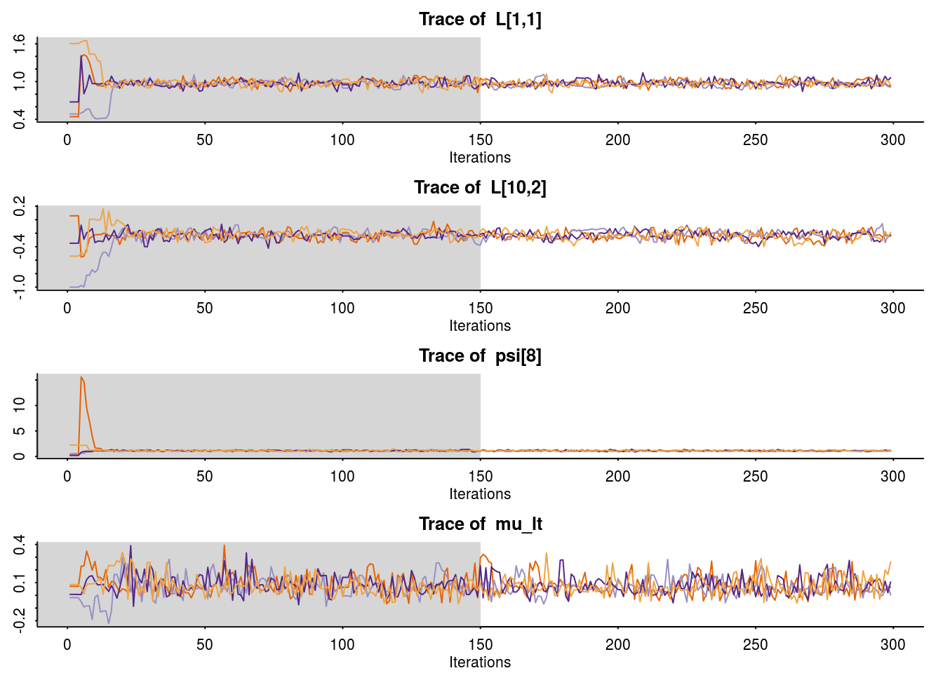
and compare with the true parameter values
print(L)## l1 l2 l3
## [1,] 0.99 0.00 0.00
## [2,] 0.00 0.90 0.00
## [3,] 0.25 0.25 0.85
## [4,] 0.00 0.40 0.80
## [5,] 0.80 0.00 0.00
## [6,] 0.00 0.50 0.75
## [7,] 0.50 0.00 0.75
## [8,] 0.00 0.00 0.00
## [9,] 0.00 -0.30 0.80
## [10,] 0.00 -0.30 0.80print(diag(Psi))## [1] 0.2079 0.1900 0.1525 0.2000 0.3600 0.1875 0.1875 1.0000 0.2700 0.2700Looks good!
This webpage was created using the R Markdown authoring format and was generated using knitr dynamic report engine.
(C) 2015 Rick Farouni
References
Algina, J. (1980). A note on identification in the oblique and orthogonal factor analysis models. Psychometrika, 45, 393–396.
Anderson, T. W., & Rubin, H. (1956). Statistical inference in factor analysis. In Proceedings of the third berkeley symposium on mathematical statistics and probability (Vol. 5, p. 1).
Bekker, P. A. (1989). Identification in restricted factor models and the evaluation of rank conditions. Journal of Econometrics, 41.
Browne, M. W. (2001). An overview of analytic rotation in exploratory factor analysis. Multivariate Behavioral Research, 36, 111–150.
Dolan, C. V., & Molenaar, P. C. (1991). A comparison of four methods of calculating standard errors of maximum-likelihood estimates in the analysis of covariance structure. BMSP British Journal of Mathematical and Statistical Psychology, 44, 359–368.
Howe, W. G. (1955). Some contributions to factor analysis (pp. 85–87). Oak Ridge, Tenn.: Oak Ridge National Laboratory.
Joreskog, K. G. (1973). A general method for estimating a linear structural equation system. Uppsala.
Kaiser, H. F. (1958). The varimax criterion for analytic rotation in factor analysis. Psychometrika, 23, 187–200.
Loken, E. (2005). Identification constraints and inference in factor models. Structural Equation Modeling: A Multidisciplinary Journal, 12, 232–244.
Lord, F. M., & Novick, M. R. (1968). Statistical theories of mental test scores (p. 532). Reading, Mass.: Addison-Wesley Pub. Co.
Millsap, R. E. (2001). When trivial constraints are not trivial: The choice of uniqueness constraints in confirmatory factor analysis. Structural Equation Modeling, 8(1), 1–17.
Thurstone, L. L. (1947). Multiple factor analysis.